“Fit” walkthrough – Circle packing, noise fields, and Joe Jackson

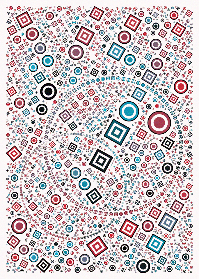
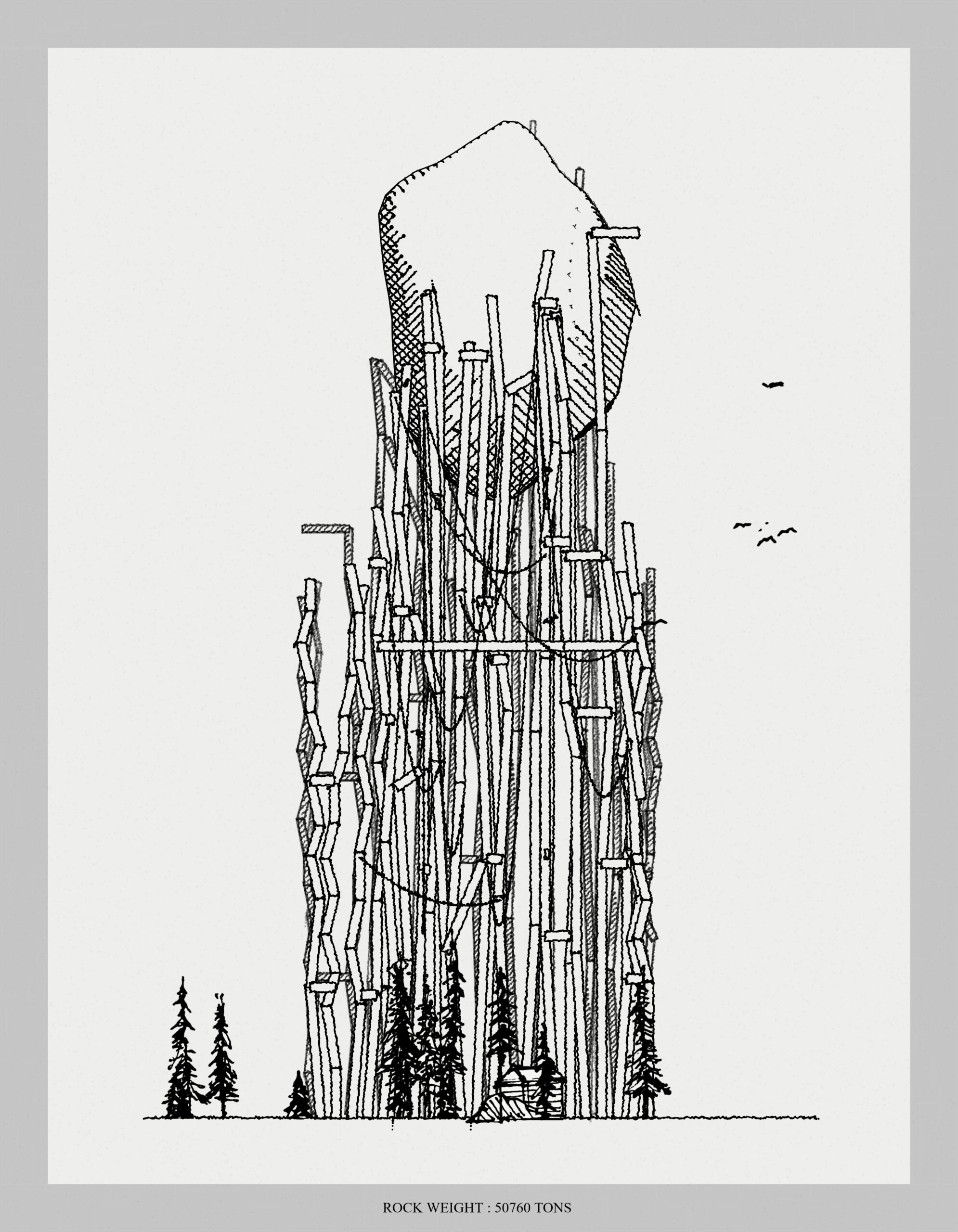
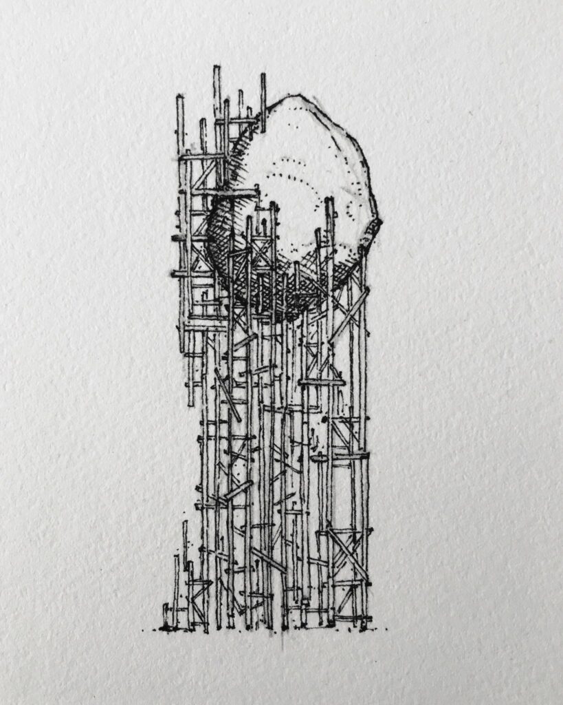
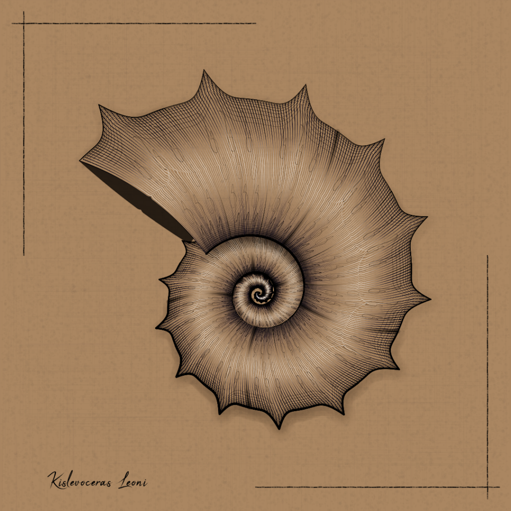
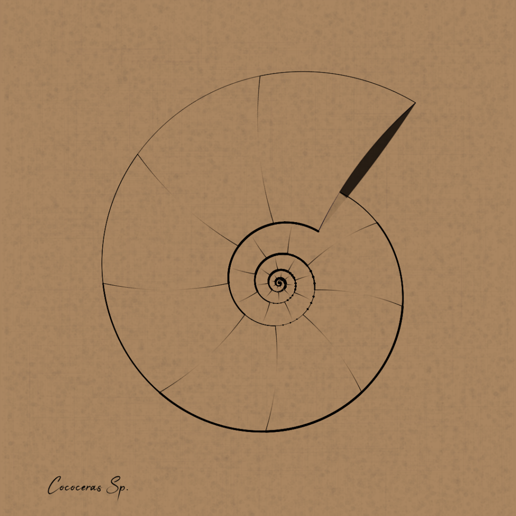
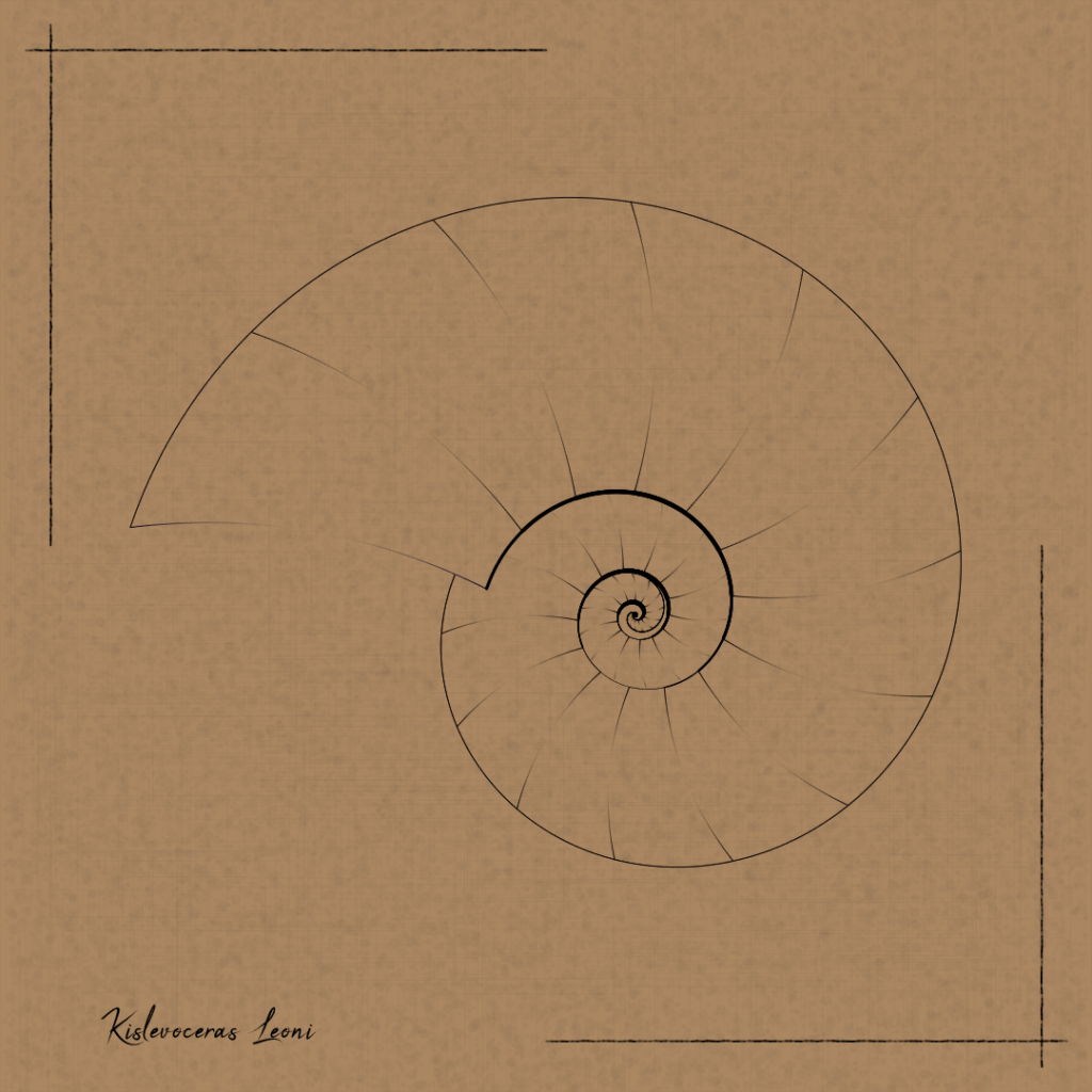
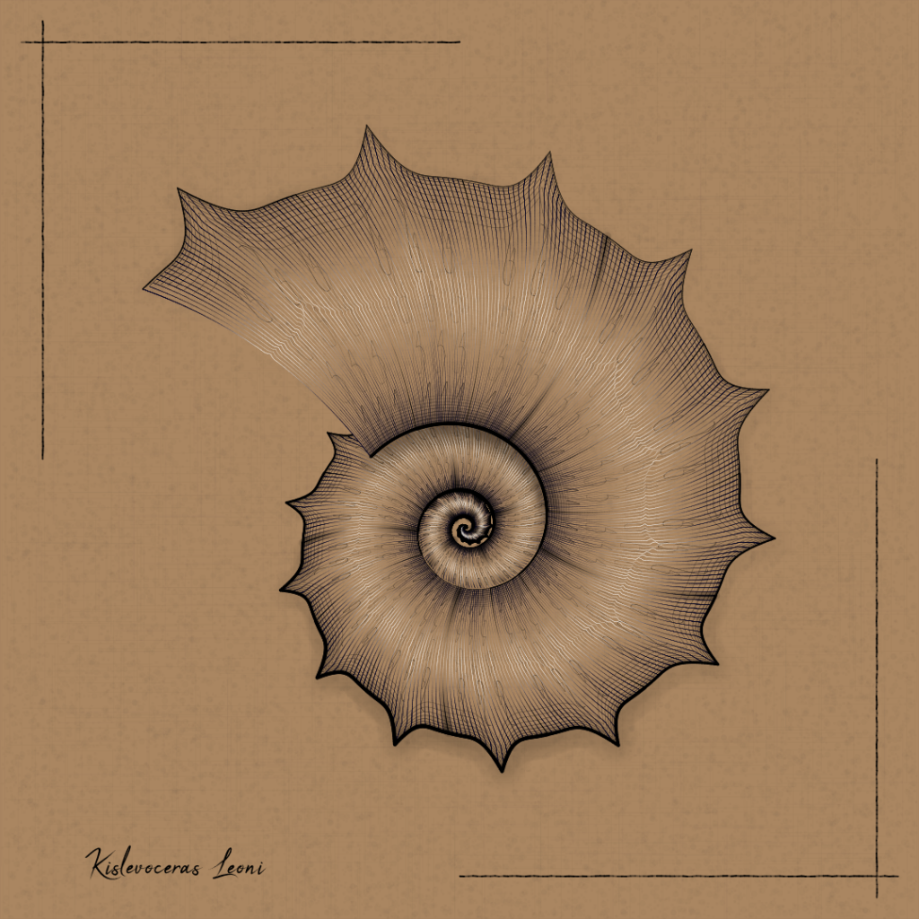
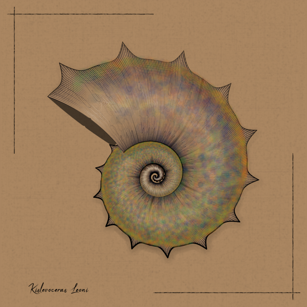
My new project “Fit” is minting as a free open edition on Base, for the entire month of June 204. Get yours here.

As I was listening to Joe Jackson’s song “Fit”, the line “Square pegs in square holes” hit home and gave me the idea to ‘fit’ square shapes on a canvas in a creative way.
That’s how inspiration often goes 🙂

(By the way, give that song a spin – it’s very modern despite being from 1980)

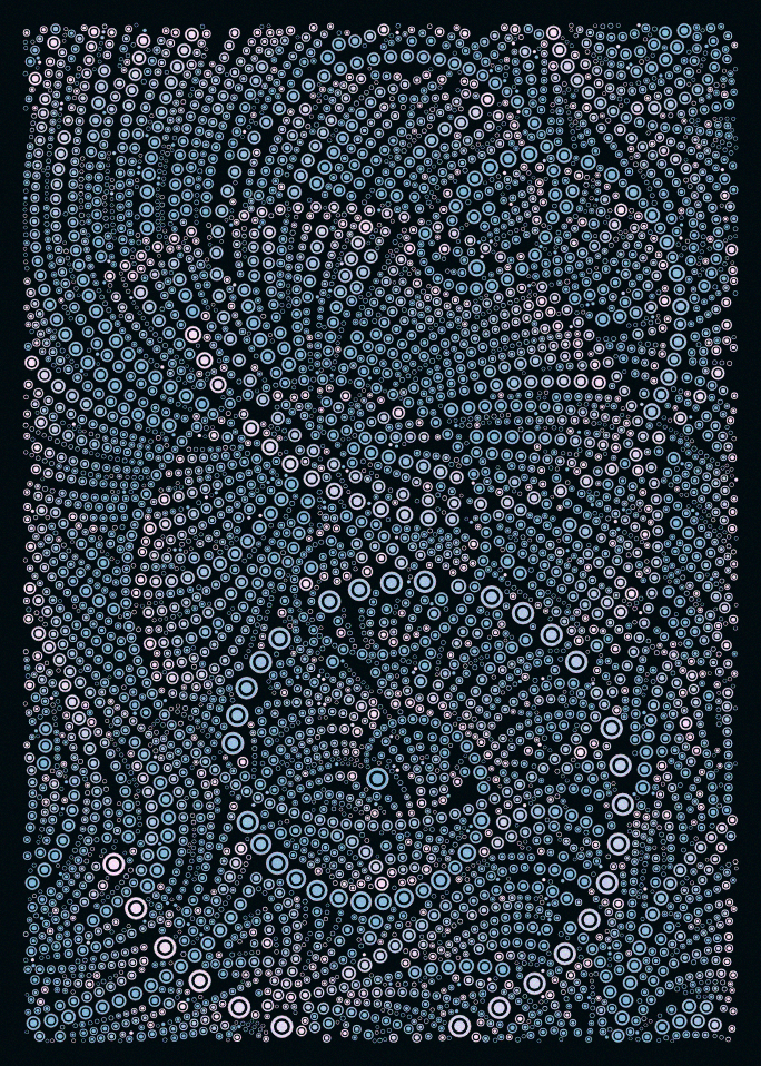
The most remarkable thing about this project, is how fast it renders. Generating a new output is pretty much instant. This walkthrough explains the main techniques that make this possible. It mostly relies on circle packing, which is one of my favorite techniques that I have used in several projects, most notably in “Circle Of Life”.

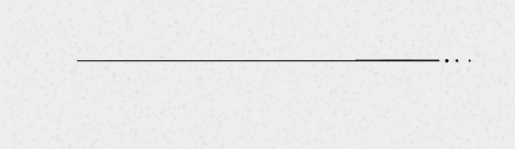
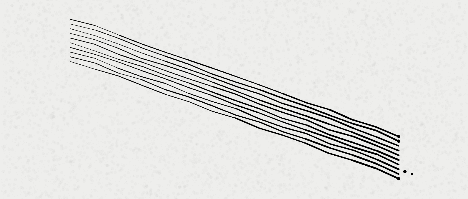
Drawing things along a noise field

Noise fields are a fairly common technique, that the master Tyler Hobbs has described much better than I’ll ever will. The core logic is, define a noise field, and map the 0-1 noise value at any given point
to a 0..360 rotation angle that gives you the direction to go for things at that particular location.

The only original part in my version, is how I implemented the noise. The classical way to implement a noise field is:

  • fill a N x N grid with random values.
  • the value at a fractional position is computed by interpolating between the 4 corner values. Various interpolation methods are common, but the typical one uses smoothsteps to ensure
    there are no sharp edges when crossing from one cell to the next.

The classical method has a number of drawbacks:

  • it uses quite a bit of memory for large N
  • if you want several noise fields, it needs even more memory – one grid per field.
  • it is periodic as you wrap around between N and 0. You can’t make an infitely varying noise field with it.

Here is my own tiny implementation that avoids all of the above problems:

let imul=Math.imul;var smoothstep0=r=>r*r*(3-2*r),fract=r=>r%1,lerp=(r,e,t)=>r+(e-r)*t;let mulberry32=r=>{r|=0;var e=imul((r=r+1831565813|0)^r>>>15,
1|r);return((e=e+imul(e^e>>>7,61|e)^e)^e>>>14)>>>0};const hash2=(r,e,t)=>mulberry32(mulberry32(r+t)+e)/4294967296,noise2d=(r,e,t,h)=>{e*=h,t*=h;var
l=fract(e),s=e-l,a=smoothstep0(l),m=fract(t),u=t-m;return lerp(lerp(hash2(s,u,r),hash2(s+1,u,r),a),lerp(hash2(s,u+1,r),hash2(s+1,u+1,r),a),smoothstep0(m))};

My method comes from the fact that you don’t really need a grid, all you need is a repeatable way to compute the random values at the 4 integer corners.
You can use a hash function to compute these and avoid the need for a precomputed grid entirely. The resulting code is ridiculously small, first we use one of the common hash functions such as mulberry32:

let mulberry32 = (a) =>
{
	a |= 0; a = a + 0x6D2B79F5 | 0;
	var t = imul(a ^ a >>> 15, 1 | a);
	t = t + imul(t ^ t >>> 7, 61 | t) ^ t;
	return ((t ^ t >>> 14) >>> 0);
};

Then we define a 2d hash function that returns a repeatable ‘random’ number for an integer (x,y) pair:

const hash2 = (x, y, seed) => mulberry32(mulberry32(x + seed) + y ) / 4294967296

And finally, given a predefined random number unique to the field (“seed”), the point coordinates (x,y) and a scaling factor k that controls the turbulence of the result, the 2d noise function is simply:

const noise2d = (seed, x, y, k) =>
{
  x *= k; y *= k;
  var fx = fract(x);
  var ix = x - fx;
  var fx0 = smoothstep0(fx);

  var fy = fract(y);
  var iy = y - fy;

  return lerp(
    lerp(hash2(ix, iy, seed), hash2(ix + 1, iy, seed), fx0),
    lerp(hash2(ix, iy + 1, seed), hash2(ix + 1, iy + 1, seed), fx0),
    smoothstep0(fy));
};

You can even make a 3D version, if you need such a thing:

const noise3d = (seed, x, y, z, k) =>
{
	var fz = fract(z);
	var iz = z - fz;
	var fz0 = fz;//smoothstep0(fz)

	var offset = iz * 1000 + 0.5;

	return lerp(
    noise2d(seed, x + offset, y + offset, k),
    noise2d(seed, x + offset + 1000, y + offset + 1000, k),
    fz0);
};

Preventing collisions

Drawing a lot of circles on the screen without collisions is, in theory, very simple: keep track of all the circles drawn so far, and adjust the radius of circles so they don’t collide with any previous one.

The basic version is something like this:

for (var i=0; i<ncircles; ++i)
{
    var c = randomCircle();
    for (var j=0; j<circles.length; ++j)
    {
        if (!circlesIntersect(c, circles[j]))
        {
            circles.push(c);
        }
    }
}

It works fine, but gets excruciating slow as you draw more and more smaller circles.

In order to speed things up, we need to limit the number of loop iterations. A really good way is to partition the space so we only run the tests on the circles in the vicinity of the one we are trying to add.

My preferred method is to split the canvas into a grid. The size of grid cells is determined so it is smaller than the largest possible circle radius.
When adding a circle to the grid, we store it based on its center coordinates – and we are guaranteed that any circle intersecting with it, has to be within the same cell, or one of the 8 neighboring cells.

Here is the code for such a circle-based grid:

// a grid for circles only. Circles are { x,y,r}
// Grid cell size = 2* maxCircleRadius, so a circle intersects at most 9 cells

class Grid {
    constructor(W, H, maxRadius) {
        var maxDiameter = 2 * maxRadius;
        this.w = (W / maxDiameter) | 0; 
        this.h = (H / maxDiameter) | 0; 
        this.W = W; 
        this.H = H;
        this.clear_();
    }

    getGridIndexForCircleCenter_(c) // return index of circle center
    {
        var i1 = clamp((this.w * c.x / this.W) | 0, 0, this.w - 1);
        var j1 = clamp((this.h * c.y / this.H) | 0, 0, this.h - 1);
        return i1 + j1 * this.w;
    }

    count_() 
    {
        var res = 0;
        this.a.forEach((v) => res += v.length);
        return res;
    }

    insert_(c) 
    {
        this.a[this.getGridIndexForCircleCenter_(c)].push(c);
    }
    
    clear_() 
    {
        this.a = [];
        for (var i=0; i<this.w * this.h;++i)this.a[i] = [];
    }

    remove_(c) 
    {
        var idx = this.getGridIndexForCircleCenter_(c);
        var a = this.a[idx];
        var index = a.indexOf(c);
        if (index != -1) 
        {
            a[index] = a.at(-1); 
            a.pop(); 
        }
        else
        { 
            console.log("invalid index found !");
        }     
    }

 
    // return true if there's at least one intersection.
    hasIntersection_(c) 
    {
        var idx = this.getGridIndexForCircleCenter_(c);

        // idx = i + j * this.w;
        var j = (idx / this.w) | 0;
        var i = idx - j * this.w;

        var x1 = (i > 0) ? -1 : 0;
        var x2 = (i < this.w - 1) ? 1 : 0;

        var y1 = (j > 0) ? -1 : 0;
        var y2 = (j < this.h - 1) ? 1 : 0;

        // this looks like a scary double loop, but the ranges are at most -1..1, so this tests at most 9 cells.
        for (var x = x1; x <= x2; ++x)
            for (var y = y1; y <= y2; ++y)
                if (this.a[idx + x + y * this.w].find(e=>circleIntersectsCircle(e,c))) return true;

        return false;
    }
}

and with this grid class, the basic code above becomes something like:

for (var i=0; i<ncircles; ++i)
{
    var c = randomCircle();

    if (!grid.hasIntersection_(c)) 
    {
      grid.insert_(c);
    }
}

It’s pretty much the same as before, but it can now handle a very large number of circles without breaking a sweat. This (and the use of vanilla js instead of P5.js) is the secret behind “Fit” blazingly fast rendering speed.

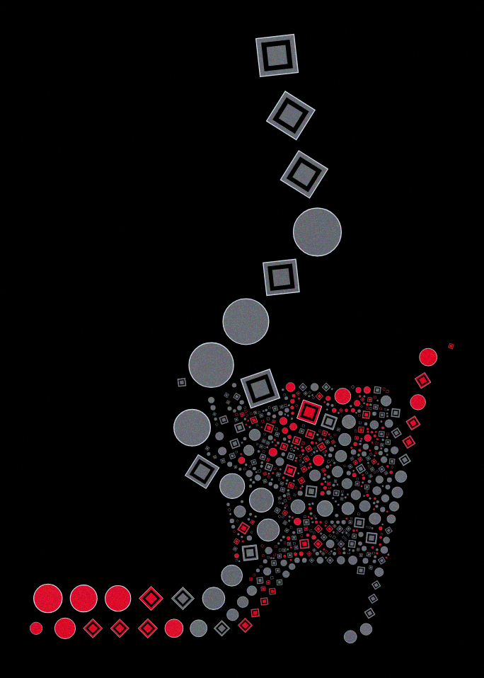
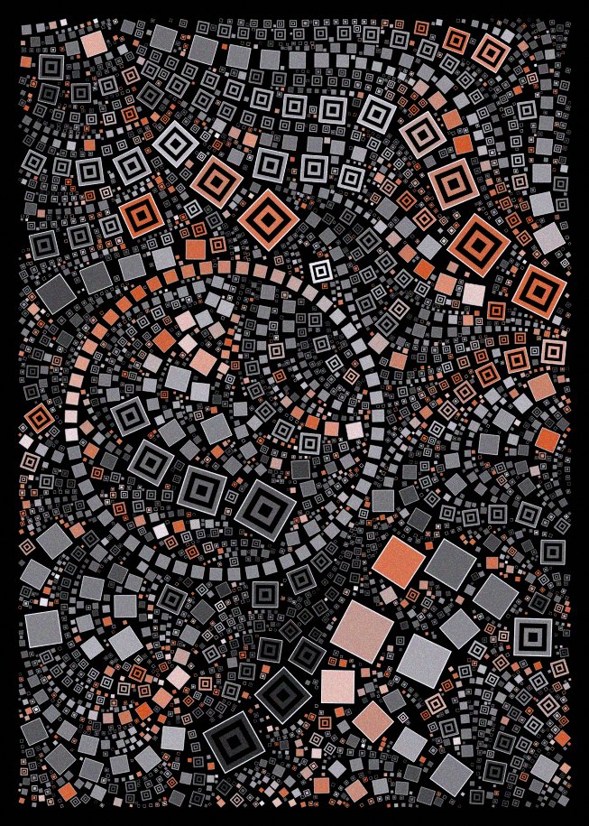
Now, in this project, I am drawing not only circles, but also squares rotated at an arbitrary angle. This complicates things a bit, as it needs tests for circle / circle, square / square, or circle / square intersections.
Circle / circle tests are very fast, so I’m leveraging the circles-based grid, by storing rotated squares using their enclosing circle + a rotation angle. This way, I can perform the fast intersection tests first.

The logic is like this, for example to test the intersection between a circle and a square:

  • first test the circle vs. the circle enclosing the square.
  • If these don’t intersect, then there’s no intersection.
  • If these intersect, then test the circle vs. the circle inscribed in the square.
  • If these intersect, then there’s an intersection.
  • Otherwise perform the costly circle / square intersection test

A similar logic is applied to speed up the tests between 2 arbitrarily rotated squares.

Putting it all together

Armed with a noise field and a fast grid-based collision detection algorithm for circles and rotated squares, the main loop of the algorithm then looks like this:

for (var i=0; i<10000; ++i)
{
	var start = pickRandomPoint();
	var circles = collectCirclesFrom(start);
	renderCircles(circles);
}

pickRandomPoint picks a random point in the canvas
collectCirclesFrom returns an array of {x,y,r} describing circles along the flow field, passing through the given start point. The logic for this is:

  • place a circle at {x,y} using a large radius. Decrease the radius as needed until that circle doesn’t collide with any other circles in the grid.
  • generate the next circle by moving x and y along the noise field, by a distance equal to the radius of the circle we just placed.
  • go on until we reach the end of the canvas, or we are unable to add a new circle.

This will generate an array containing a nice stream of circles starting from the start point. Then we do the same, from the same start point, but reversing direction. This gives us a second array.
We reverse that second array, and append the first one to it – and this gives us the full list of circles to draw.

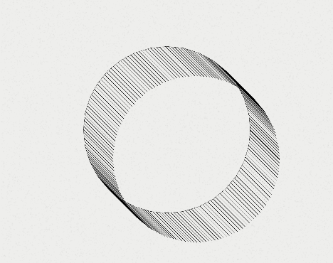
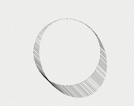
In order to make things a little more interesting with the noise fields, I decided to add random ‘attractors’ to the noise field logic. These are spatial regions that distort the noise field around them. Each attractor has an intensity, distortion angle, and direction (so it can push the field away instead). Combining these is a good way to breathe new life into the (somewhat overused)
noise field effect, with interesting spirals, nodes and swirls.

Generative color palettes

I wanted to keep the code size as small as possible, so I used a generative color palette system. Instead of using a predefined list of colors,
I used a seed for a random number generator and generated colors based on a set of rules. Predefined palettes were stored by generating thousands of these palettes, and curating the ones
I liked best. The beauty of this system is that I was able to store a palette using just its seed, which its a big size improvement compared to a list of specific colors.

For this project I ended up curating 100 different palettes. Most of the times, the generated ones were pleasing enough, so I also kept a rare option to use a fully random palette.

The rules for generating the colors were as follows:

  • decide if the palette is using a dark or light background. Depending on this, set the background to black and foreground to white, or the other way around.
  • generate up to 24 colors. A single color is generated by picking 10 random colors, and keeping the one that has the largest sum of distances to all the other colors generated so far. There
    is also a threshold value that eliminates colors that are too close to an existing one.
  • adjust the foreground and background, by interpolating them slightly towards one of the colors in the generated list.
  • depending on the threshold, sometimes only 2 grey colors are generated. In that case, generate extra shades of grey, interpolated towards a random hue.
  • finally, remove a random number of colors from the list

This logic generates palettes where the colors try to maximize their relative distance to each other. I experimented with different ‘distance’ algorithms. Strangely, the clever ones that used
perceptual color adjustments, created worse palettes than the basic one that just adds the square of the differences between the r,g,b components. I also tried other colorspaces but it didn’t
improve things significantly, so in the end I stayed with the simple RGB version.

Artistic choices

At that point, I had a nice engine that could render packed circles along a noise field fairly fast. This is that sweet time where the technical side takes a backseat to the artistic side: “how can I use this to make cool looking things” ?
I love that phase, and can often get stuck in it, experimenting with options, for months.

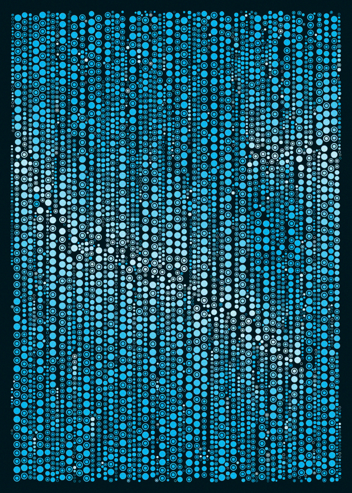
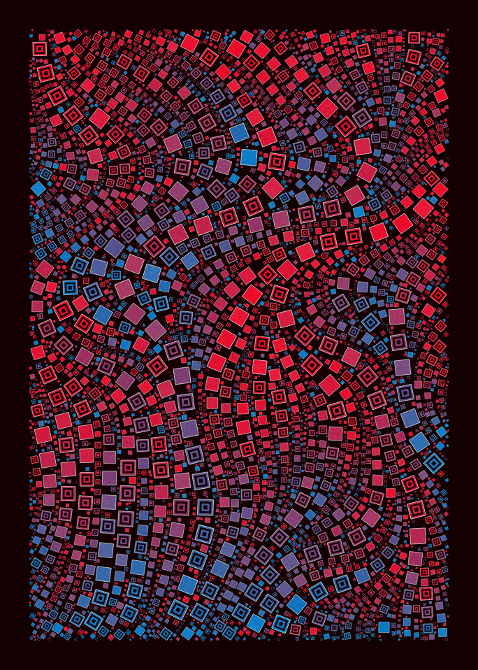
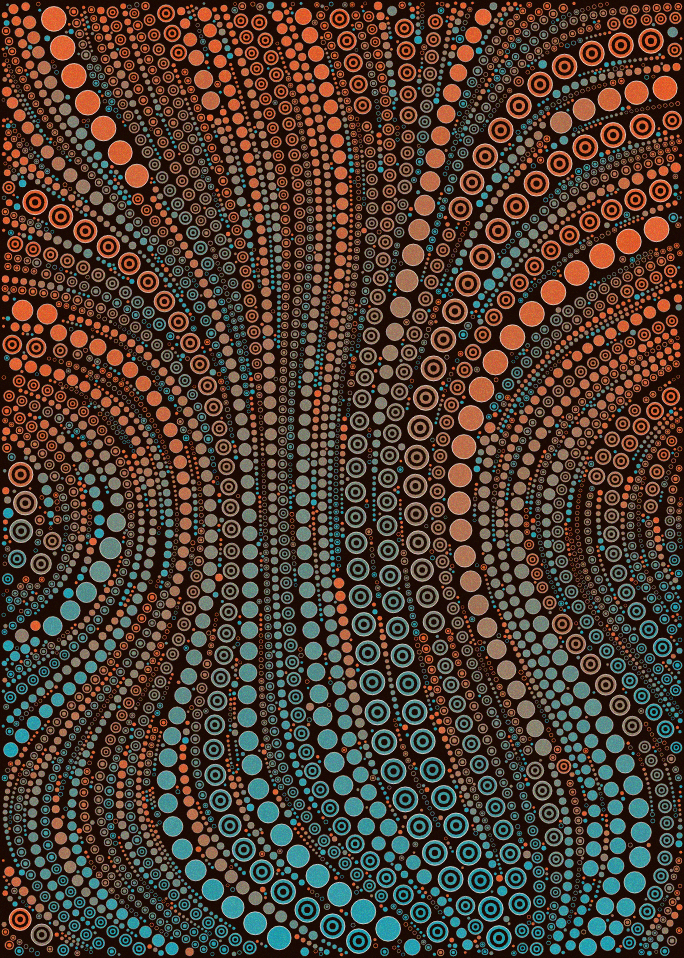
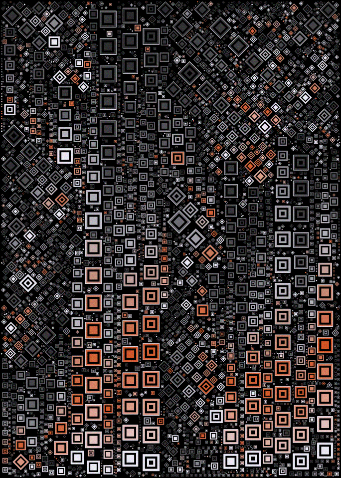
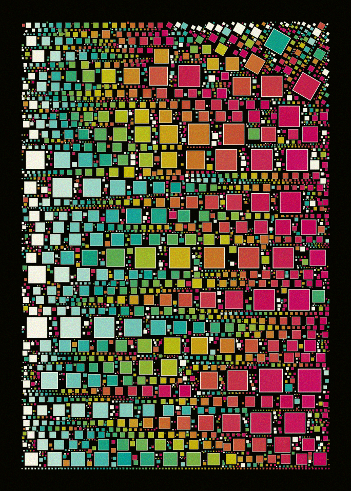
There are a number of options that let the program generate outputs with a nice amount of variability. Here are the main ones.

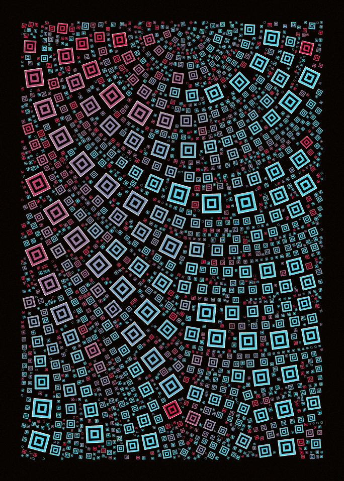
  • items rendering: circles and squares can be rendered as solid shapes, or using several levels of nested shapes (a nod to QQL). They can also have extra spacing for a more sparse layout.
    the chose shape can change at every item drawn, or be kept the same for a given call to renderCircles(). Square shapes can have a fixed angle, or turn along to follow the field.
  • items size range: the shapes have a random range for their allowed sizes, which creates variations between very dense outputs with thousands of tiny shapes, to more abstract ones with larger shapes.
  • color allocation: when rendering the array of circles, colors can span the full color palette, or only a random subset of it. Colors can also be quantized to the selected palette range, or use a gradient between palette colors.
  • initial points selection: pickRandomPoint() can, in some case, limit the selection of initial point to a few large random rectangles or circles. Having less freedom for picking up a starting point, the resulting
    piece is often more sparse, with larger empty areas.
  • maximum length along the field: collectCirclesFrom() can limit the number of circles to a random value.
  • dual field: in some cases, I used 2 different noise fields, picking one or the other in collectCirclesFrom()
  • field quantization: the 0-360 angle given by the noise field, can be quantized to sharp angles.
  • initial circles and spirals: in some iterations, before placing circles along the noise field, I also start by placing shapes along larger circles or spirals. This occupies some of the space
    in a less predictable way.

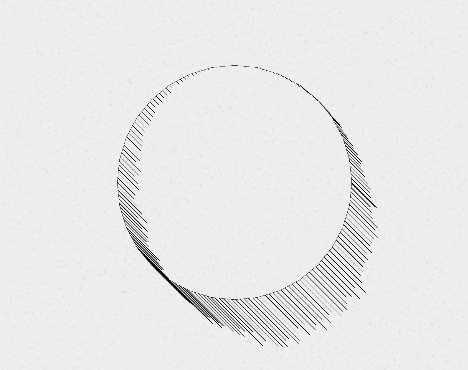
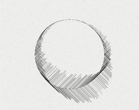
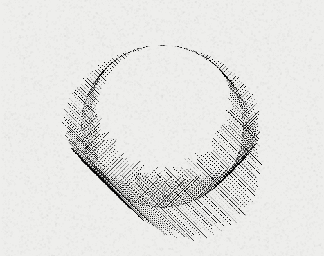
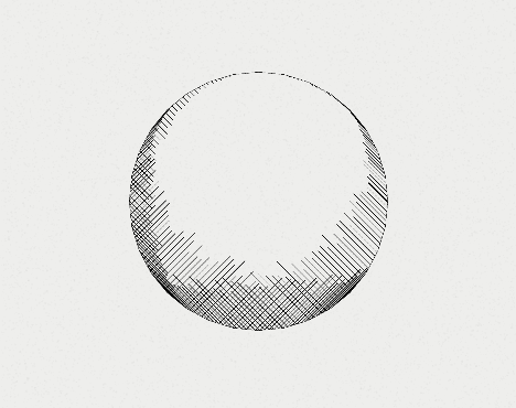
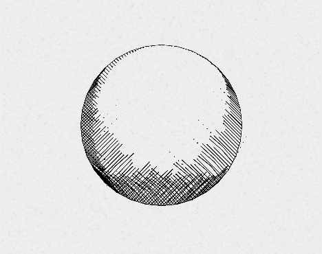
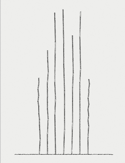
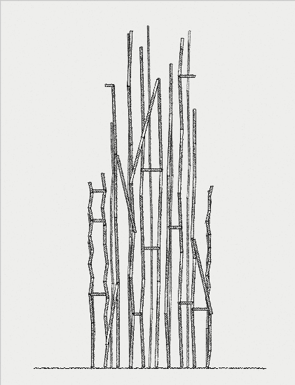
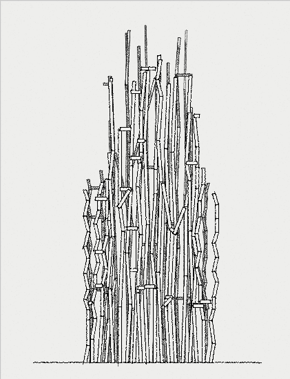
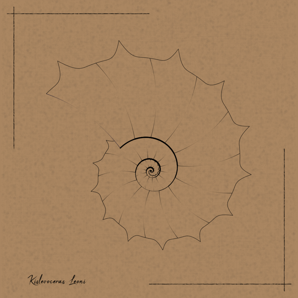
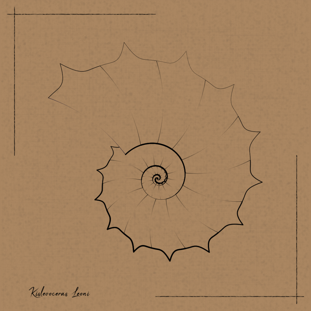
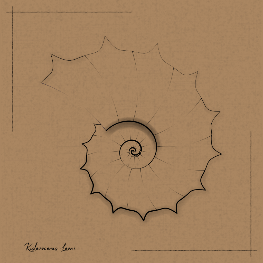
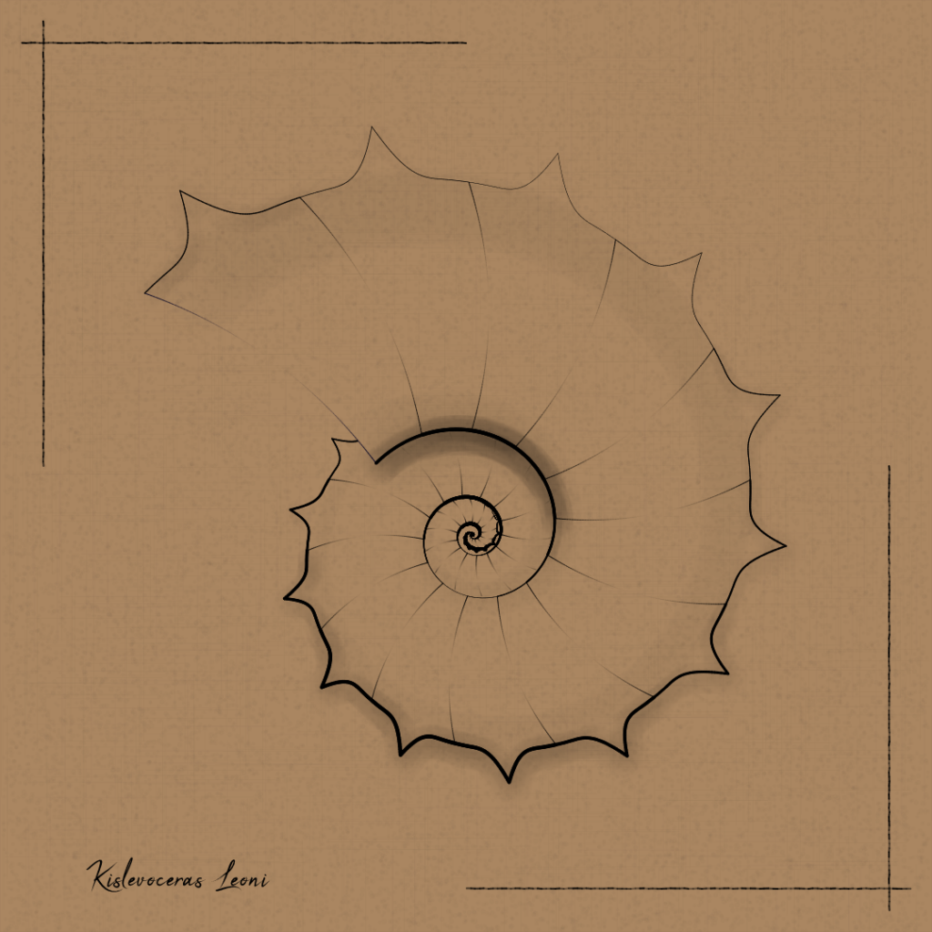
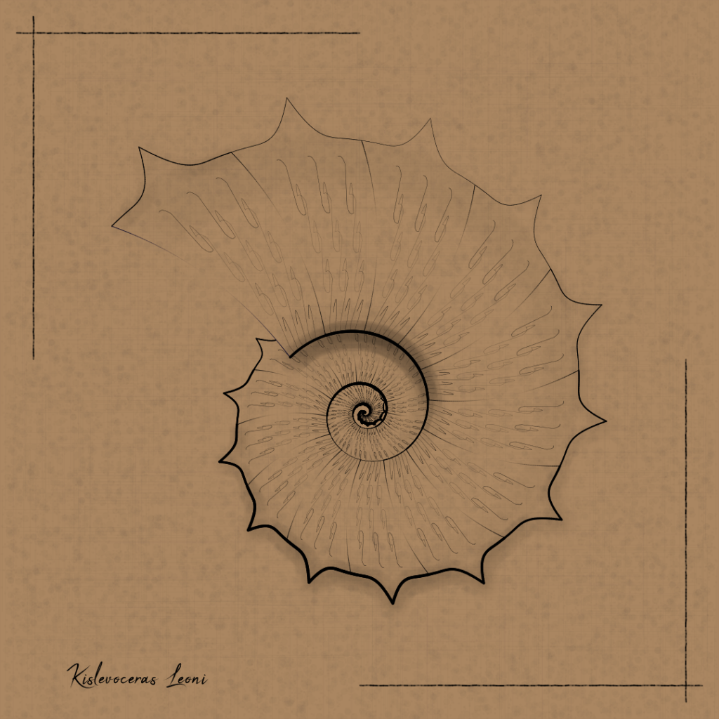
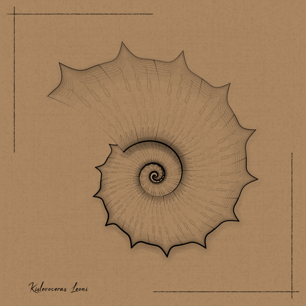
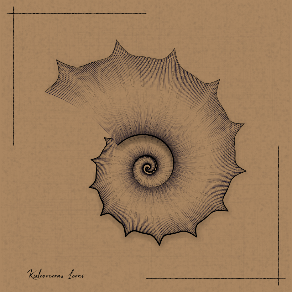
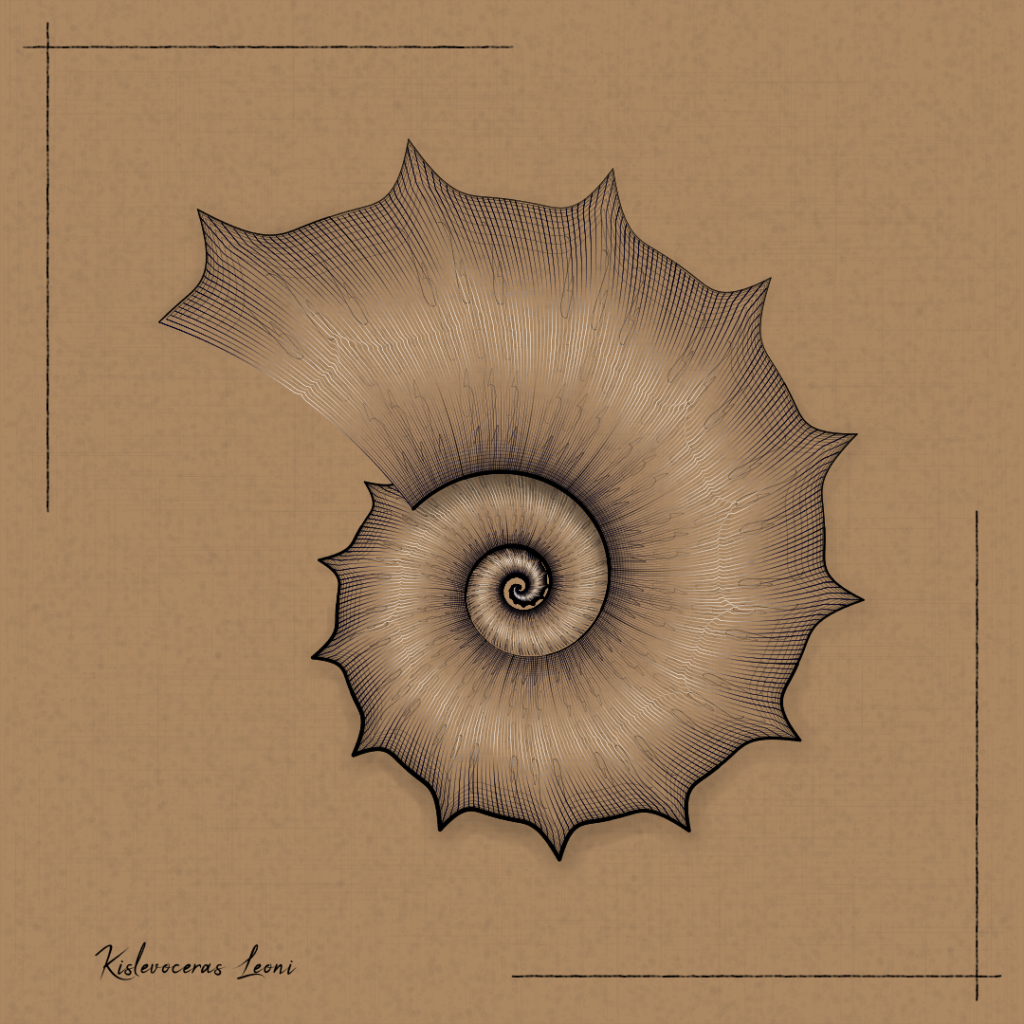
I’ll leave you with a few sample outputs illustrating some of these options, with a wave to all my misfit friends out there…

Initial spirals occupying the space
1-direction quantization of the field
Spawning area constraints
Noise field attractor
Picking between 2 different fields
Circles only
Quantizing in 3 directions
2 fields, one direction quantize
2 circles initial occupation

Making of “Circle Of Life”

This week I finally released my “Circle Of Life” project on Alba. The feedback has been unbelievable so far !
I have received a lot of questions about the code, in this post I will try to answer the most frequent ones.

Inspiration

The project got largely inspired by this blog post by Gorilla Sun. “A Recursive Circle Packing Algorithm for Organic Growth Patterns”. Even though I didn’t use any of Gorilla’s code, the beautiful examples made me think, “what if I made a system of circular cells, growing organically using circle collision” ? That’s how “Circle Of Life” was born.

The project is really about starting with a circular cell, and applying a set of rules, driven by probabilities, to let this cell grow, die, or spawn new cells. As the project evolved, more complex rules were added, cells were rendered in fancier ways instead of using plain circles, but the core principle stayed the same: grow circular shapes until they don’t have any room left to grow.

Growing circles

Growing a circle is usually just a matter of increasing its radius. However, in our case we want the cell to grow from whatever location it was spawned from – so when the circle grows, its radius increases and its center moves in the opposite direction of the spawn point. The formula is:

center = spawnPoint + k * (center-spawnPoint)

where k is the ratio between the old radius and the new radius.


Even though the project ended up using vanilla js and WebGL, it is often useful, in the early stages, to prototype using p5.js.


The code below is a p5.js sketch that forms the core, non-optimized algorithm of “Circle Of Life”.

const W = 800;
const H = 800;
const START_RADIUS = 3.0; // start radius
const DIVIDE_RADIUS = START_RADIUS * 3; // start dividing after that radius
const GROWTH_DELTA = 1; // increase radius by that amount at each step
const SPAWN_PROBABILITY = 0.05; // probability to spawn a child circle
var circles = [];

// circles intersect if the distance between the centers is less than the sum of radiuses
var circlesIntersect = (c1, c2) => 
{
	var dx = c1.x - c2.x;
	var dy = c1.y - c2.y;
	var d2 = dx * dx + dy * dy;
	var sr = c1.r + c2.r;
	return d2 < sr * sr;
};

// check if circle c intersects another circle, ignoring the one at index 'except'
var intersectAny = (c, except) => 
{
	for (var i = 0; i < circles.length; ++i) 
	{
		if (i != except && circlesIntersect(circles[i], c)) return true;
	}
	return false;
};

// create a new circle of radius r, tangent to circle c0 at angle alpha
var newCircle = (c0, alpha, r) => 
{
	var c =
	{
		x: c0.x + (r + c0.r) * Math.cos(alpha),
		y: c0.y - (r + c0.r) * Math.sin(alpha),
		r: r,
		canGrow: true
	};
	c.ox = c0.x + c0.r * Math.cos(alpha);
	c.oy = c0.y - c0.r * Math.sin(alpha);
	return c;
};

function setup() 
{
	createCanvas(W, H);
	circles.push(newCircle({ x: W / 2, y: H / 2, r: 0 }, Math.random() * TAU, START_RADIUS));
}

var drawCircles = () =>
{
	fill(255);
	stroke(0);
	strokeWeight(1);

	for (var i = 0; i < circles.length; ++i) 
	{
		var c = circles[i];
		circle(c.x, c.y, 2 * c.r);
	}
};

var inFrame = (c) =>
{
	return c.x >= 0 && c.x < W && c.y >= 0 && c.y < H;
};

function draw()
{
	background(0xff);
	drawCircles();

	var done = true;

	for (var i = 0; i < circles.length; ++i) 
	{
		var c = circles[i];
      
        // attempt to grow this circle
		if (c.canGrow)
		{
			var oldx = c.x, oldy = c.y, oldr = c.r; // save these in case growing the circle causes a collision
			var k = (c.r + GROWTH_DELTA) / c.r; // growth factor
			c.x = c.ox + k * (c.x - c.ox);
			c.y = c.oy + k * (c.y - c.oy);
			c.r *= k;
          
            // if the new circle intersects another circle, revert
			if (intersectAny(c, i))
			{
				c.canGrow = false;
				c.x = oldx; c.y = oldy; c.r = oldr;
			}
			else
			{
                // if the new circle is in frame, we're not done
                // otherwise it can't grow any more
				if (inFrame(c)) done = false;
				else c.canGrow = false;
			}
		}

        // if this circle is large enough, it has a probability to spawn a child
		if (c.r >= DIVIDE_RADIUS && Math.random() < SPAWN_PROBABILITY)
		{
            // If after 100 attempts, we couldn't spawn a child that doesn't collide
            // with other circles, give up.
			for (var n = 0; n < 100; ++n)
			{
                // note the 1.02 factor. Without it, rounding errors cause the 2 circles to be detected as intersecting too early.
				var child = newCircle(c, Math.random() * TAU, START_RADIUS * 1.02);
				if (!intersectAny(child, i))
				{
                    // this child doesn't collide with other circles. Add it to the list
					child.r = START_RADIUS;
					circles.push(child);
					c.canGrow = false; // parent circle can't grow any more
					done = false;
					break;
				}
			}
		}
	}

	if (done) 
	{
		console.log("done");
		noLoop();
	}
}


Life cycle of a cell

In the example above, cells grow and spawn until they run out of space. For this project I really wanted to focus on death as a necessary part of life, so the life cycle of cells was based on actual living organisms:

  • Cells grow until they run out of space, or reach a predefined ‘old age” size.
  • Once cells reach a predefined “maturity” size, they have a probability of spawning new cells.
  • Once a cell stops growing, it has a predefined lifespan. Once this lifespan is exceeded, the cell starts dying.
  • Dying cells shrink at a predefined rate, until they reach a 0 radius, at which point they are removed from the list.

With nothing more than the above parameters, very interesting results were achieved. Depending on old age / maturity / lifespan, the system would colonize the whole canvas and quickly die, or slowly evolve and move through the available space in mesmerizing wave-like patterns.

Adding variety

In order to make things visually more interesting, I defined several types of cells:

  • “Default” cells behave as described above
  • Sometimes, instead of spawning a child cell, a cell creates “Spore” cells. These are tiny cells that move away quickly from the parent in a explosion-style fashion. Friction forces are applied so that after reaching a certain distances, these spore cells turn into Default cells, and start growing as well.
  • Another feature is called “Side-shoots” cells. When a parent spawns a side shoot, this new cell doesn’t grow in size, but in turn, spawns another side shoot. This goes on until a given length has been reached, and the last side shoot turns into a default cell.
    Parents can spawn any number of side shoots, from 1 to 64. Large number of side shoots create flower-like patterns.
    To complicate things further, side shoots also have a probability to split into 2 side shoots, creating branches.
    Side shoots are not spawn at random locations, but instead, follow a noise field.

Each piece has its own unique probability for spores, side shoots, branching, number of side shoots per parent, …

Optimizing collisions

As the piece was taking shape it quickly became obvious that the naive O(n^2) collision detection system in the code above, was a big bottleneck and had to be optimized.

I first made a version using quadtree-js. It worked great, but had 2 drawbacks: first, it added almost 2Kb to the code (an important thing to consider when releasing on ETH). And second, it was actually too general. Quadtrees are great for managing arbitrary sized rectangles with random distributions. But in the case of “Circle Of Life”, the shapes are all circles, and are always distributed evenly (since they aren’t allowed to overlap). So a simpler structure can be used !

After trying out various options, I settled for the simplest one: subgrid partitioning. The main grid is divided in 100×100 smaller grids, and each grid stores a reference to the circles that intersect with it. Then, testing if a circle overlaps with other circles is limited to all the grids containing the considered circle. This allowed me to achieve close to 60fps, even with very busy grids.

Rendering with WebGL

At that point the drawing itself was starting to be the bottleneck. WebGL to the rescue !

The rendering is very much inspired by this example: the GL_POINTS primitive is used to pass all the circles in one single call to the GPU. Each point has its own gl_PointSize, allowing to draw many different sized cells at once. Then a fragment shader renders all these points, usually by overlapping various circles drawn using signed distance functions. In the case of the “Amoeba” style, the point is rendered using the classical “metaball” effect, which is achieved by combining the SDF’s of various moving circles.

Generative music

As the visuals were very relaxing and meditative, I decided to add a generative ambient soundtrack to the piece. I used Tone.js (mostly because it was available on ETHFS).

As you may know, I’m not new to ambient music, having released a couple albums on Bandcamp and Spotify. In that case, it was all about working with limitations. Size was the main constraint, ruling out the use of samples, so all the sounds had to be dynamically generated. I built a mixer system on top of Tone.js so I could use familiar concepts such as buses and effect loops.

For ambient music, 2 things are critical: there has to be very little tension in the music, and at the same time, there has to be constant motion. I tried to achieve this in different ways. In terms of composition, the system picks a key, then either a major or minor triad from that key. These 3 notes get sent to 3 harmony channels (so I don’t need to deal with polyphonic synths, it’s 3 mono synths) where their pan and levels get automated with various lfos. I use a spread voicing so the triad covers 2 octaves and doesn’t clutter a narrow range.
This already gives a lot of animation, but hearing the same 3 notes for 5 mn gets very boring. So the next trick is to add a bass note underneath, and change that bass note while the triad stays the same. Changing the bass note creates minor 7 or major 7 chords, which are perfect for ambient since they hold no tension by themselves.

Finally I routed all the channels except the bass one to to buses for reverb, delay, pitch shifters, using circular patching to create complex feedback loops (like it is done with modular synths).

Lastly, I generated events from the visuals when spawning side shoots or spore cells. These trigger extra melody notes picked randomly between the 3rd, 7th or 9th of the current chord.

Closing words

It took several months of fine tuning things to get it to that final release, but it was definitely worth it ! The initial concept had most of the code already, but adding details was the fun part (and the tedious one as well).

I was overwhelmed by the reception of this project, and I want to thank all the collectors for their support.

Please feel free to ask on Twitter (X) if you want more details about any specific part of the project. If you’re an artist, keep doing what you’re doing, and enjoy the process !

1d4393b-7ed85683-2b198780-672e3f76-1

Mining Structures walkthrough

Laxraven and I just released our collaborative project “Mining Structures” on FxHash. It was a huge success, and I have received many questions about the process and techniques used. Here is a quick walkthrough.

The project started with a failure. @Laxraven had posted a beautiful architectural drawing on Twitter, and someone mentioned they would love to see a generative version – to which I foolishly replied, “Challenge accepted”.
As it turned out, this initial drawing was pretty difficult to convert to generative. Peter had used very aggressive, loose lines in his sketch, and my initial attempts at emulating these were, well, not that great. So after some discussions we decided to recreate a different piece that would be more suitable. I chose his “Structure holding object” drawing:

“Structure holding object” by @laxraven

Analog lines

Looking at the details of the original drawing, it was quickly obvious that I needed a way to draw lines with a natural feel to them. Peter’s line are never perfectly straight, some of them have little splatters of ink at the end of the line, or little ink bubbles… So the first step was to write a “natural line engine” in P5.js. I would share the code, but I’m a big adept of “teach a man/woman to fish” principle, so I would rather deconstruct the logic and see what others come up with. If you really want the code, it is on the blockchain.

Here are the features I ended up with. In the examples below I am drawing a straight horizontal line.

“analogueness” – this splits the line in a lot of different points (the longer the line, the more points) and displaces each of them randomly. A javascript function is used to control the line weight across the progress of the line.

“Analogueness” feature
// color function = black the whole way
var cfunc = (idx, p) => color(0); 
// weight function = randomized, but increasing
var wfunc = (idx, p) => ((1+8*idx+3*rnd())/W); 
var lineDrawer = new LineDrawer(cfunc, wfunc);
// how often to split, and how much to displace
lineDrawer.setAnalogueness(0.1, 0.01);
// draw horizontal line
lineDrawer.draw(vec2(-0.7, 1.05), vec2(0.7, 1.05));

end bubble probability” – this controls the probability that the line ends with a little ink ‘bubble.

“end bubble” feature
// draw line straight
lineDrawer.setAnalogueness(0.1, 0.0);
// with a bubble at the end
lineDrawer.setEndBubbleProbability(1.0);

“splatter probability” – this controls the probability that the line has little ink splatters at the end. They typically increase in distance and shrink in size. I have parameters to control the minimum line length before splatter occurs, the maximum splatter distance, the splatter probability and the maximum number of repetitions.

// draw line straight
lineDrawer.setAnalogueness(0.1, 0.0);
// with splatter at the end
lineDrawer.setSplatter(10/W, 40/W, 1.0, 5, 1.25);

When combining all the feature together, we get some lovely organic flow with very little code:

lineDrawer.setAnalogueness(0.1, 0.01);
lineDrawer.setEndBubbleProbability(0.3);
lineDrawer.setSplatter(10/W, 40/W, 0.1, 5, 1.125);
for (var i=0; i<10; ++i)
{
lineDrawer.draw(drawingLayer, vec2(-0.7, 0.5-0.02*i), vec2(0.7, -0.02*i));
}

Shading

“How did you do the shading on the rock ?” is probably the most frequently asked question. Again I’ll deconstruct it, using a circle as an example.

1. draw lines along the circle in the SE direction

2. adjust the line lengths based on their position on the circle

3. Randomize line lengths a bit

4. Do it again in the NE direction.

5. And again in the NW direction

5. Clip drawing to the original circle

6. Turn on “analog line drawing” features

Drawing the scaffolding

With the line drawing engine in place, this part was rather straightforward. I drew it in 3 layers with various levels of transparency to give it a sense of depth. Each layer is made of vertical rectangles of random heights that are randomly split and displaced.

First layer
First+second layers
All 3 layers

Drawing the ropes

These were not in the original drawing, but we decided they would add a nice textural change to the piece.
They are made by picking random pairs of points within the scaffolding (or the main rock) and drawing a parabola between them. The parabola is adjusted so the middle point has the same height than the lowest point in the pair. This made the math somewhat easy to deal with.

Adding analog elements

The generative drawing was starting to look pretty good at this point, but it took another dimension entirely once we added analog elements on the ground line. Laxraven drew several trees, houses, and rocks using ink on paper, scanned them, and we mixed them with the generated drawing, taking special care to match the line weights so they would blend seamlessly. This really perfected the illusion, making it very difficult for the viewer to distinguish the analog elements from the generated ones.

During this last phase we also spent a lot of time adding rarity features, such as a random crack in the rock, sometimes filled with gold or opal colors, as well as the ultra-rare “frog” rock.

This project was a lot of fun and I’m looking forward to the next collab with Laxraven !

Here are a few images from the series (including some outtakes from the development that didn’t make it into the final collection).
You can also view the full collection in its high resolution glory (and generate an infinity of variations) at fxhash.

3a1c7f609ae94e0000-3b081bd43d41460000-4a5f18ab4905cc0000-2fa431b5b889b80000-scaled

Image 1 of 11

3f164ec6eba0a20000-87433af5e671b8000-468eb9aed731a00000-31a68a146eb7ea0000

Ammonites walkthrough

Following the unexpected success of the Ammonites NFT on fxhash, several people have asked me to give more information about my approach for producing this type of generative pieces.

So here it is, I’m going to take this image and deconstruct it for you, step by step.

1. The easy part first – the background paper

The background canvas is generated with noise and random vertical / horizontal lines. With exaggerated contrast and in greyscale, it looks like this:

The code for generating these is fairly simple:

function noise_pattern(layer, fg,bg, N, ll)
{
	layer.fill(bg);
	layer.stroke(fg);
	layer.strokeWeight(1.0 / layer.width);
	layer.rect(-1, -1, 2, 2);

	ll = ll / layer.width * (1.0+rnd());
	for (let i = 0; i < N; i++)
	{
		let x1 = rrnd(-1 + ll, 1 - ll);
		let y1 = rrnd(-1, 1);
		let x2 = rrnd(-1, 1);
		let y2 = rrnd(-1 + ll, 1 - ll);
		
		layer.circle(x1, y1,ll);
	}
}

function canvas_pattern(layer, fg, bg, N, ll)
{
	layer.fill(bg);
	layer.stroke(fg);
	layer.strokeWeight(1.0 / layer.width);
	layer.rect(-1, -1, 2, 2);

	ll = ll / layer.width * (1.0+rnd());
	for (let i = 0; i < N; i++)
	{
		let x1 = rrnd(-1 + ll, 1 - ll);
		let y1 = rrnd(-1, 1);
		let x2 = rrnd(-1, 1);
		let y2 = rrnd(-1 + ll, 1 - ll);
		layer.line(x1 - ll, y2, x1 + ll, y2);
		layer.line(x2, y1 - ll, x2, y1 + ll);
	}
}

backgroundLayer.background('#b08a65');
canvas_pattern(backgroundLayer, color('#00000008'), color('#b08a65'), 1000, 100);
noise_pattern(backgroundLayer, color('#00000004'), color('#00000004'), 10000, 10);
noise_pattern(backgroundLayer, color('#00000004'), color('#00000004'), 20000, 4);

Note that I normalize my canvas to -1..1 units, instead of using pixel units.

If you look closely at the frame lines, you will notice they are not perfectly straight, but are a little shaky, to imitate the feel of hand drawn lines. This is the kind of tiny detail that came in late in the development, but I feel is extremely important to add that final polish. The shaky line is drawn by subdividing the whole line in 100 segments, and applying a tiny bit of randomization to each segment point.

2. Drawing spirals

The general formula for a spiral shape is well-known, and looks like (in polar coordinates)

r = e^(b θ) – different values of b give different spiral growths.

Next, we can scale the spiral to define the inner and outer shell locations. If they overlap, it’s a classic nautilus structure. If they don’t, we get an unrolled shell.

3. Shell subdivisions

Ammonites are made of consecutive chambers. Another parameter I introduced is the “number of chambers per rotation”, i.e, how many chambers are in a 2π turn around the spiral. Here is an example with RotationSteps = 7.

This number doesn’t have to be a integer, as a matter of fact non-integer values produce more complex patterns that are visually interesting. Here is one with RotationSteps = 8.5

and our image at the top of this page, stripped down to the bare essentials, looks like this (RotationSteps = 13.58)

4. Outer spiral decoration

Now that our shell is defined with an outer and inner edge, we can add decorations (spikes, knobs, ridges, …) to the outer edge.
For each chamber we have an index that goes from 0 to 1, and a ‘decoration function’ that produces the various decoration types.

For example here is a function that produces a spike in the middle of the chamber:

function addMiddleSpike(x, w, amount)
{
	if (x < 0) x = 0;
	else if (x > 1) x = 1;
	if (Math.abs(x - 0.5) < w)
	{
		var t = (1.0 - Math.abs(x - 0.5) / w);
		return t * t * t * amount;
	}
	return 0;
}

The various functions for producing the decorations are fairly simple, have quite a few parameters, and when combined together, provide a huge variety of designs with a lot of room for randomization – ideal for generative designs !

Here is our initial image, with its outer decoration applied:

5. Line weight control

This step is so crucial that I feel it deserved a paragraph on its own. Traditional artists (working with ink) add a lot of variation to their lines thickness. So far our drawing looks very flat, so let’s make the outer spiral lines thicker at the bottom, and thinner at the top, and do the opposite for the inner spiral lines:

It’s a subtle difference, but all these little details compound in the end !

6. Drop shadows

This one is rather straightforward, I used the HTML canvas drop shadow features. P5.js doesn’t expose these, so we need to work with the device context directly. I vary the alpha of the shadow based on the distance from the center, and only draw the shadows for the last turn of the spiral.

const stepThreshold = RotationSteps * 2 | 0;
drawingLayer.drawingContext.shadowBlur = 24;
drawingLayer.drawingContext.shadowOffsetX = 3; 
drawingLayer.drawingContext.shadowOffsetY = 6; 
var shadowAlpha = (step > stepThreshold) ? 10 * (step - stepThreshold) : 0;
if (shadowAlpha > 200) shadowAlpha = 200;
drawingLayer.drawingContext.shadowColor = color(0, 0, 0, shadowAlpha);

7. Spiral shadow

Let’s add some sense of volume to our otherwise flat spiral, by drawing some more shadows around the edges. I basically walk around the spiral, drawing almost transparent circles with a brush that increases in size.

function drawShadows(nsteps)
{
	drawingLayer.push();
	drawingLayer.noStroke();
	drawingLayer.fill(color('#00000002'));

	var brushSize1 = function (x)
	{
		return 0.001 + 0.05 * x * x * x * x * x;
	}
	var brushSize2 = function (x)
	{
		return 0.001 + 0.2 * x * x * x * x * x;
	}
	draw_function_with_circle_brush(drawingLayer, function (x)
	{
		return outerSpiral(stepToAngle((nsteps - 0.1) * x)).smul(0.99);
	},
		brushSize1, 500, 100, 500);
	draw_function_with_circle_brush(drawingLayer, function (x)
	{
		return outerSpiral(stepToAngle((nsteps - 0.1) * x)).smul(0.92);
	},
		brushSize2, 500, 100, 499);

	draw_function_with_circle_brush(drawingLayer, function (x)
	{
		return innerSpiral(stepToAngle((nsteps - 0.1) * x)).smul(1.01);
	},
		brushSize2, 200, 50, 199);

	drawingLayer.pop();
}

and here is the end result:

8. Suture patterns

Ammonites have decorative suture patterns, which are textural lines separating the chambers. There are many different types of suture patterns, and I wish I had spent more time on these, as some of the patterns on the actual fossils are exquisitely intricate. I used simple parametric equations to draw 2d curves along the radial axis. Having several equations allowed me to add more entropy to the collection.

Here is our picture, with its suture patterns drawn.

9. Contour hatching

That was the hardest part to get right. I added hatching in 2 directions, first around the outer edge:

and then radially, using a variable alpha so the radial lines are transparent in the center:

Finally I also added a second radial pass, using white highlights, with alpha fading to transparent towards the edges:

10. Radial lines accents

I also added a feature to accent every N chamber separation. In our example N = 3, and it looks like this with the accents added:

11. Closing the shell

Here I close the shell by drawing a symmetrical version of the final radial line, and filling the gap with a dark color. This part was incredibly hard to get right in all cases, as the geometry around the closure can be pretty complicated with spikes and ridges… I ended up drawing the full shape on a different layer, and then using P5.js erase() mode to remove the part from the previous turn that should still be visible.

11. Magic blend trick for extra contrast

Finally, to add more contrast to the final image, I used P5.js blend() in SOFT_LIGHT mode, blending the image onto itself. This gave it this extra pop you can see in the picture at the top of the page.

12. Rare “ammolite” version

Some ammonites are made of an opal-like mineral that’s absolutely beautiful. I tried to recreate the effect in a very small (~4 %) number of editions. I picked colors from actual ammolite stone, and blended them over the shell contour with variable transparency and brush sizes.

I think it’s nice to add rare features like this, as people who mint one of these get really excited and generate a lot of buzz.

13. Closing notes

In conclusion, for this type of illustrations I believe that the devil is really in the details. All these little things that you can barely see individually, all add up to elevate the piece.

I had a lot of fun designing this, even though towards the end, I was seeing spirals in my sleep !

For any questions, hit me up on Twitter or FxHash discord.